In this tutorial, we dive into the power of Polygon.io's Flat Files for downloading and analyzing trade-level data across the entire stock market on a specific day. While the Trades API excels at fetching detailed trades for specific tickers at precise times, Flat Files streamline the process of acquiring an extensive dataset, enabling analysis that spans all trades for an entire day with just a single download. This guide aims to illustrate how Flat Files can unlock both wide-ranging market insights and the intricate details of trade-level data, providing a comprehensive toolset for deep market analysis.
Getting started with Flat Files for Market Analysis
Flat Files are included in all paid plans, providing immediate access to historical market data in a compressed CSV format. After signing up for an API key with a supporting stocks subscription, you have two main options for downloading data:
File Browser: The web-based File Browser offers an intuitive interface for accessing and downloading historical market data directly. No additional tools or downloads required.
S3 Access: Ideal for automating data retrieval tasks within your software or scripts. See our knowledge base for setup instructions.
Exploring the Structure of Flat Files
Each Flat File contains a day's worth of market activities, including detailed trade data, across all tickers. Here's a snippet to illustrate the file structure:
These files capture every trade for all stocks on the specified day, offering a source of truth for all market activity.
Understanding Trade Data Attributes
The real value in Flat Files lies in the depth of data provided for each trade across the entire market in a single file. Attributes like
conditions
,
exchange
, and
price
give insights into the specifics of each transaction, while aggregated data can reveal broader market trends. What is really neat though is when you start to aggregate trades together you can build a much better understanding of the market. By dissecting the structure of this data, we gain deeper insights into the nuances of each trade event. In this section, we will explore each attribute of the trade data object and its significance.
Conditions (
conditions
): A list of condition codes that provide additional context or modifiers about the trade, such as whether it was an odd lot, a split trade, or executed during a trading halt.
Correction (
correction
): Indicates the trade correction status. This is particularly relevant when trades need adjustments or corrections post-execution.
Exchange (
exchange
): Identifies the exchange on which the trade was executed. The values are integer-based, and you can refer to Polygon.io's Exchanges documentation to map these IDs to their respective exchange names.
Trade ID (
id
): A unique identifier for each trade. Uniqueness is maintained based on a combination of the ticker symbol, the executing exchange, and the Trade Reporting Facility (TRF).
Participant Timestamp (
participant_timestamp
): A high-precision Unix timestamp denoting when the trade was generated at the exchange. This timestamp provides nanosecond accuracy, capturing the exact moment the trade was executed.
Price (
price
): Reflects the price at which the trade was executed. When multiplied by the trade's size, this gives the total dollar value of the trade transaction.
Sequence Number (
sequence_number
): An increasing sequence number that establishes the order of trade events for a particular ticker. While these numbers are increasing, they may not always be sequential and will reset each trading day.
SIP Timestamp (
sip_timestamp
): Another high-precision Unix timestamp, but this one denotes when the SIP (Securities Information Processor) received the trade from the exchange.
Size (
size
): Represents the volume of the trade, i.e., how many shares were exchanged in that particular trade event.
Tape (
tape
): A categorization based on which exchange the ticker is listed on. The tapes are:
Tape A: NYSE listed securities
Tape B: NYSE ARCA / NYSE American
Tape C: NASDAQ
TRF ID (
trf_id
): An identifier for the Trade Reporting Facility where the trade was executed. This provides more granularity about where the trade was reported.
TRF Timestamp (
trf_timestamp
): A high-precision timestamp showcasing when the trade was received by the Trade Reporting Facility.
In sum, the intricacies of the trade data structure provide a comprehensive view of market transactions, each attribute offering a different perspective into the world of trading. But, aggregating this data can uncover patterns such as peak trading times and preferred exchanges, enriching our understanding of market behavior.
From Individual Trades to Aggregated Insights
Now that you have seen how Flat Files work, let’s dive into the actual data and explore. First, let's download an actual file and explore the data and see what we can learn. We start by downloading the trades for 2024-04-05 via the File Browser.
The
us_stocks_sip/trades_v1/2024/04/2024-04-05.csv.gz
file is about 1.35GB and is in a compressed gzip format. So, let’s
gunzip
it.
$ gunzip2024-04-05.csv.gz
This command results in a CSV file approximately 6.2GB in size, ready for analysis. Now, let’s see the file structure using the
head
command:
$ head -n 42024-04-05.csv
ticker,conditions,correction,exchange,id,participant_timestamp,price,sequence_number,sip_timestamp,size,tape,trf_id,trf_timestamp
A,"12,37",0,11,52983525035312,1712306654208705342,142.99,3807,1712306654208740096,5,1,0,0A,"12,37",0,11,52983525035313,1712306654208705342,143,3808,1712306654208743168,8,1,0,0A,12,0,11,52983525035314,1712306654429439337,143,3809,1712306654429468160,187,1,0,0
You can see here the file contains over 70 million trades.
$ wc -l 2024-04-05.csv
70,399,9142024-04-05.csv
So, we have just over 70 million trades but how many ticker symbols are contained in this file? The following command counts the total number of unique ticker symbols in the first column of the "2024-04-05.csv" file, excluding the column header "ticker".
But, say for example, you wanted to see how many trades
TSLA
had, you could run something like this:
$ grep TSLA 2024-04-05.csv | wc -l
1,549,605
We did a preliminary exploration using command-line tools to get a sense for what’s contained in this file, now let’s transition to a more detailed analysis through Python scripting. Python is amazing for data analysis and we can drill down into specific aspects of the market activity.
Here’s a Python script for analyzing the dataset, that identifies the top 10 most traded stocks and calculates their respective percentages of the total trades (code here).
TSLA: 1,549,605 trades, 2.20% of total trades
NVDA: 788,331 trades, 1.12% of total trades
SPY: 669,762 trades, 0.95% of total trades
AMD: 587,140 trades, 0.83% of total trades
MDIA: 561,698 trades, 0.80% of total trades
AAPL: 540,870 trades, 0.77% of total trades
SOXL: 533,511 trades, 0.76% of total trades
QQQ: 508,822 trades, 0.72% of total trades
CADL: 466,604 trades, 0.66% of total trades
AMZN: 465,526 trades, 0.66% of total trades
You can see here
TSLA
,
NVDA
, and
SPY
emerge as the most traded stocks, underscoring their significance in the day's trading activity.
What about if you wanted to look at the distribution of trades across different exchanges? Well, let’s use a similar python script (code here).
Exchange4: 25,570,324 trades, 36.32% of total trades
Exchange12: 15,147,689 trades, 21.52% of total trades
Exchange11: 6,877,306 trades, 9.77% of total trades
Exchange19: 5,098,852 trades, 7.24% of total trades
Exchange10: 4,006,611 trades, 5.69% of total trades
Exchange8: 3,686,168 trades, 5.24% of total trades
Exchange15: 2,446,340 trades, 3.47% of total trades
Exchange21: 2,173,744 trades, 3.09% of total trades
Exchange7: 1,509,083 trades, 2.14% of total trades
Exchange20: 1,296,811 trades, 1.84% of total trades
Exchange18: 674,553 trades, 0.96% of total trades
Exchange13: 527,767 trades, 0.75% of total trades
Exchange2: 417,295 trades, 0.59% of total trades
Exchange3: 393,919 trades, 0.56% of total trades
Exchange17: 230,210 trades, 0.33% of total trades
Exchange1: 183,010 trades, 0.26% of total trades
Exchange9: 159,020 trades, 0.23% of total trades
Exchange14: 1,211 trades, 0.00% of total trades
This illustrates the market's backend infrastructure, with exchanges
4
and
12
dominating trading volume, indicating its central role in market operations. You can learn more about exchanges using the Exchange API.
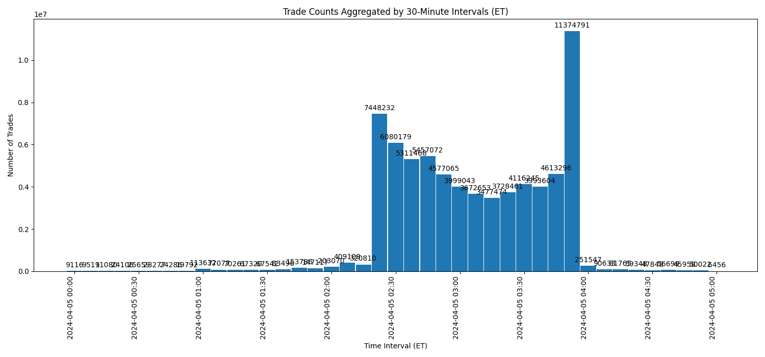
Understanding Market Hours
The stock market's trading day is divided into three key phases: pre-market, regular market, and after-hours trading, each with distinct characteristics and volumes. Notably, within the regular market the initial 15 minutes after the market opens and the final 15 minutes before it closes are often the busiest times, reflecting heightened trading activity as traders react to overnight news or prepare for the next day.
Pre-Market Trading (4:00 AM - 9:30 AM ET): During pre-market hours, investors react to news and reports released overnight, leading to potential volatility due to lower liquidity compared to regular hours.
Regular Market Trading (9:30 AM - 4:00 PM ET): This period experiences the highest volume, with the first and last 15 minutes marking the peaks of activity as traders seek to establish or close positions based on the latest market developments.
After-Hours Trading (4:00 PM - 8:00 PM ET): Similar to pre-market, after-hours trading allows for reactions to late-breaking news with the caveat of reduced liquidity and potentially greater price fluctuations.
To visualize these dynamics, we can use a Python script to create a histogram aggregating trades into 30-minute intervals (code here), providing a clear view of when trading activity concentrates during the day. This analysis aims to highlight the distribution of trading volume across the day, from pre-market to after-hours.
The resulting histogram vividly illustrates the intensity of trading activity throughout the day. Peaks during the opening and closing periods of the regular trading session underscore the critical windows of heightened market activity, aligning with our expectations of busy periods. Meanwhile, the visualization also brings into focus the relative calm of mid-day trading and the contrasting volumes seen during pre-market and after-hours sessions.
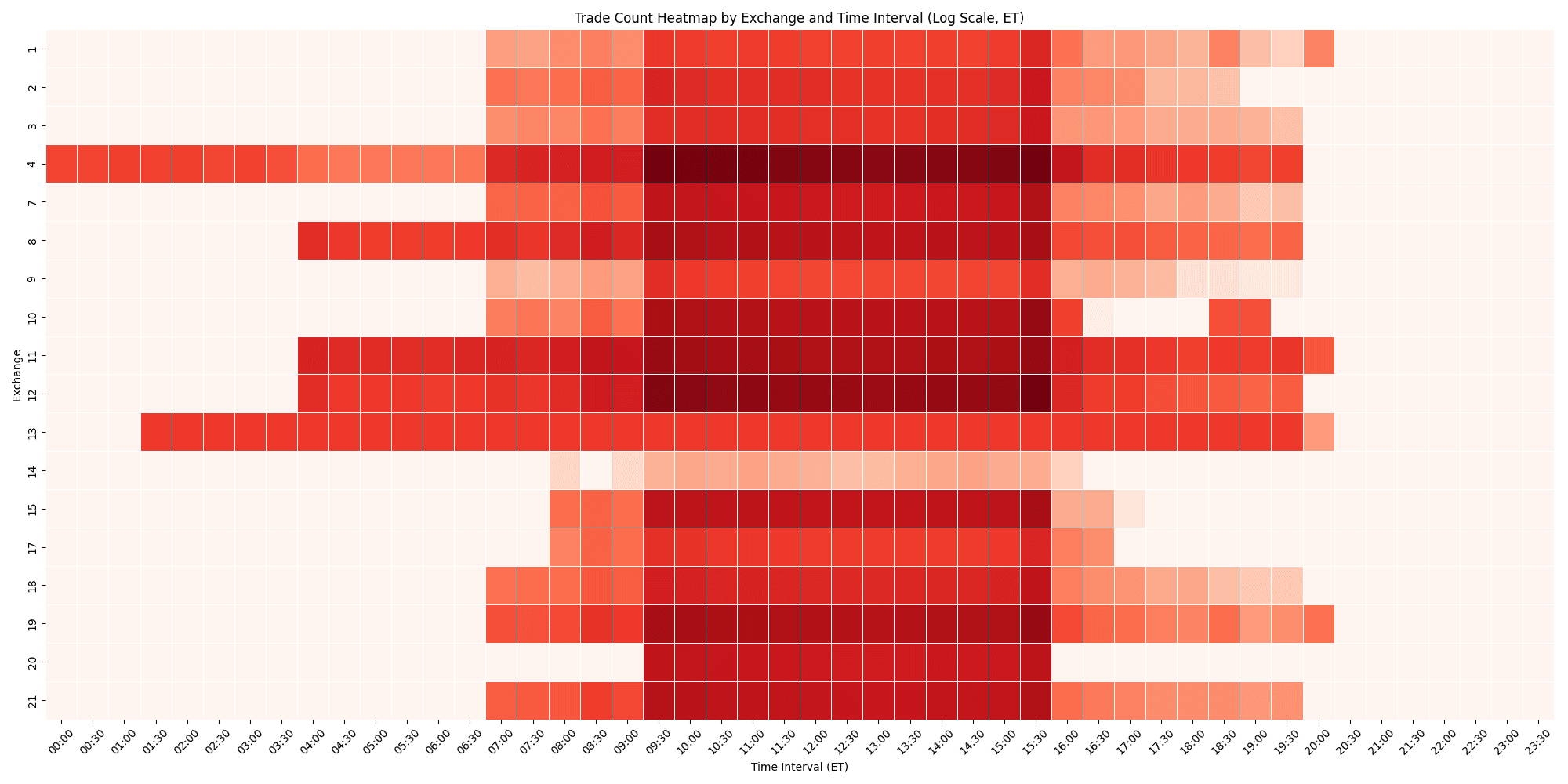
Analyzing Trade Volumes Across Exchanges
For many, the term 'stock market' conjures up images of a singular, unified marketplace where shares are traded en masse. In reality, the stock market is not just one entity; it's a decentralized system composed of multiple exchanges. When an order to buy or sell a stock is placed, it can be routed to any one of these exchanges, depending on various factors such as the time of day, type of trade, available prices, commissions, and specific routing preferences of brokers. This distribution across exchanges ensures that traders and investors have access to the best possible prices and provides a competitive landscape that encourages fair and efficient trading.
We can use a Python script that aggregates trades by exchange into 30-minute chunks, setting the stage for a visual analysis. This approach will highlight trade flows, including opening hours and peak activity times, across the exchanges (code here).
The analysis reveals much more than just the volume dominance of certain exchanges; it uncovers operational patterns and hours of operation, including earlier start times indicated by significant pre-market activity on some exchanges. Moreover, the heatmap visualization brings to light the pivotal roles of Exchanges 4 and 12, which collectively process approximately 50% of all trades, highlighting their central importance in the market's framework. These insights, from trading intensity to the strategic timing of operations across various exchanges, provide a clearer understanding of the intricate market dynamics, underlining the significance of these exchanges in facilitating a substantial portion of the day's trading activity.
Next Steps
Flat Files are a powerful tool for comprehensive market analysis, offering a seamless transition from broad market insights to detailed trade-level details without many API calls. This tutorial hopefully highlighted their utility in revealing trading patterns, from identifying peak activity times to analyzing trade volume distribution across exchanges, particularly the significant role of Exchanges 4 and 12.
Beyond simplifying workflows, Flat Files enable a depth of market analysis that is essential for informed decision-making. They allow developers and traders to closely inspect the market's mechanics, leading to optimized trading strategies and a deeper understanding of market behavior. In essence, Flat Files unlock the potential to discover the market's vastness through its intricate details, providing a foundation for data-driven insights that drive strategic decisions.
Polygon.io is excited to announce a new partnership with Benzinga, significantly enhancing our financial data offerings. Benzinga’s detailed analyst ratings, corporate guidance, earnings reports, and structured financial news are now available through Polygon’s REST APIs.
This tutorial demonstrates how to detect short-lived statistical anomalies in historical US stock market data by building tools to identify unusual trading patterns and visualize them through a user-friendly web interface.